

Linear Optimization
The task of optimization is to find the optimal value for a given objective, while satisfying given constraints.
The program determines the optimal solution for a two-variable objective function with linear inequalities as constraints.
Example 1 (Maximization)
A factory produces two different types of cell phones. X units of type A and y units of type B are to be completed daily.
- Constraints:
- The individual departments have the following daily production capacities:
- The assembly line for type A can produce a maximum of 600 units.
x ≤ 600 - The assembly line for type B can produce a maximum of 700 units.
y ≤ 700 - The plastic department can produce a maximum of 750 units. x + y ≤ 750
- The electrical department can produce a maximum of 400 type A units or 1200 type B units or a combination of both.
This means that 1/400 of the total time is required for each of type A and 1/1200 for each of type B.
1/400·x + 1/1200·y ≤ 1 or 3·x + 1·y ≤ 1200;
- The assembly line for type A can produce a maximum of 600 units.
- Objective function:
- How many units of each type must be produced per day in order to obtain maximum profit if the profit for type A is $140 per unit and for type B $80.
Objective function:
  ƒ(x,y) = 140·x + 80·y → Maximum

Constraints:
  x ≥ 0
  y ≥ 0
  x ≤ 600
  y ≤ 700
  x + y ≤ 750
  3·x + y ≤ 1200

Maximum
  x = 225   y = 525
  ƒ(x,y) = 73500
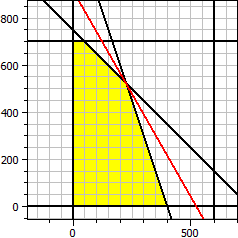
Therefor, the maximum profit of $73500 is achieved if 225 type A and 525 type B units are produced each day.
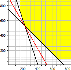
Example 2 (Minimization)
Objective function:
  ƒ(x,y) = 140·x + 80·y → Minimum

Constraints:
  x ≥ 0
  y ≥ 0
  x ≥ 160
  y ≥ 80
  x + y ≥ 750
  3 x + y ≥ 1200

Minimum
  x = 225   y = 525
  ƒ(x,y) = 73500
Note:
The conditions x ≥ 0 and y≥ 0 do not need to be entered. They are automatically added.
See also:
Setting the graphicsWikipedia: Linear programming