Growth models

Regression involves determining the unknown parameters of a growth model or a given function for a series of measurement data so that the final model fits the data as well as possible. Commonly considered models are:

Linear growth

In linear growth, the rate of change, i.e. the derivative of the growth function, is constant.
The corresponding graph is a straight line.

Exponential growth

In exponential growth, the rate of change is proportional to the population:   ƒ'(t) ∼ ƒ(t)

Limited growth

In limited growth, the rate of change is proportional to the saturation deficit, i.e. the difference between the saturation limit S  and the population:   ƒ'(t) ∼ (S − ƒ(t))

Logistic growth

Logistic growth assumes that the population initially grows essentially exponentially, but that growth slows as it approaches the saturation limit. Therefore the rate of change is assumed to be proportional to both the population and the saturation deficit. This leads to the differential equation:   ƒ'(t) = k · ƒ(t) · (S − ƒ(t))
which has the solution: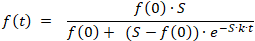

For a given saturation limit S , the program determines the initial value ƒ(0)  and the proportionality factor k  to fit the function ƒ(t)  to the given value pairs.

Method

The program determines the logistic function f(t)  in the form: 

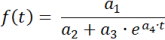
The parameters are    a₁ = ƒ(0)·S ,  a₂ = ƒ(0) ,  a₃ = S - ƒ(0) , and  a₄ = -k·S .

S  is the saturation limit, i.e. the value that the function asymptotically approaches.
ƒ(0)  is the value of the function at the point t = 0 , which is not necessarily the first measured value.

In addition, the inflection point of the function is determined, i.e. the point from which the slope decreases again.
The function value at the inflection point is always equal to half the saturation limit so  ƒ(t_w) = ½·S .
The derivative ƒ'(t_w)  at the inflection point gives the maximum growth rate,

The parameters of the logistic function are determined as follows:

1. Step: Form the reciprocal function of ƒ(t)   to get the sum from the denominator into the numerator.
2. Step: Take the logarithm of both sides to obtain the exponent t .
3. Step: Write the equation in the form h(t) = m·t + b .
4. Step: Perform a linear regression on the pairs of values  ( t  | h(t) ) .
5. Step: Reverse the transformation for  m  and  b .

Linear regression also provides the determination coefficient, the correlation coefficient and the standard deviation.